030 — Flux cycle calculation

This tutorial computes CO2 + H2O fluxes from quality-controlled chamber concentration cycles. It runs end-to-end on the bundled synthetic sample (no setup required) — set PALMWTC_DATA_DIR to point at your own QC parquet to use real data instead.

What you’ll see:

1. Resolve I/O paths (config layered: kwargs → env → yaml → bundled).

2. Run the "flux" pipeline step (under the hood: cycle identification, linear-fit slope per cycle, scoring, optional ML outlier flagging).

3. Plot the resulting per-cycle flux time series and a diurnal heatmap.

4. Inspect the cycles dataframe for downstream calibration.

import pandas as pd
import matplotlib.pyplot as plt

from palmwtc.config import DataPaths
from palmwtc.pipeline import run_step
from palmwtc.viz import set_style

set_style()
pd.set_option("display.width", 120)
pd.set_option("display.max_columns", 20)

1. Resolve I/O paths

DataPaths.resolve() walks: explicit kwargs → PALMWTC_DATA_DIR env → palmwtc.yaml → bundled synthetic sample. The last layer always succeeds, so this notebook runs even on a fresh pip install palmwtc with no setup.

paths = DataPaths.resolve()
print(paths.describe())

DataPaths (source=sample (bundled synthetic), site=libz):
  raw_dir       = /home/runner/work/palmwtc/palmwtc/src/palmwtc/data/sample/synthetic
  processed_dir = /home/runner/work/palmwtc/palmwtc/src/palmwtc/data/sample/Data/Integrated_QC_Data
  exports_dir   = /home/runner/work/palmwtc/palmwtc/src/palmwtc/data/sample/exports
  config_dir    = /home/runner/work/palmwtc/palmwtc/src/palmwtc/data/sample/config
  extras        = <none>

2. Run the flux step

run_step("flux") does the work: load QC parquet → discover chambers from CO2_C<n> columns → for each chamber, prepare data + identify cycles + fit slopes + score quality → write 01_chamber_cycles.csv.

This is one library call, fully testable, no notebook-cell-resident logic.

result = run_step("flux", paths)
print(f"Step status: {'OK' if result.ok else 'FAILED'}")
print(f"Elapsed:      {result.elapsed_seconds:.1f}s")
print(f"Rows in:      {result.rows_in:,}")
print(f"Rows out:     {result.rows_out}")
print(f"Artefact:     {result.artefacts[0]}")
print(f"Chambers:     {result.metrics.get('chambers')}")

Step status: OK
Elapsed:      16.6s
Rows in:      20,160
Rows out:     3
Artefact:     /home/runner/work/palmwtc/palmwtc/src/palmwtc/data/sample/exports/digital_twin/01_chamber_cycles.csv
Chambers:     ['C1', 'C2']

3. Inspect the cycle output

cycles = pd.read_csv(result.artefacts[0])
print(f"{len(cycles)} cycles across {cycles['chamber'].nunique()} chamber(s)")
cycles[["chamber", "cycle_id", "flux_date", "flux_slope", "r2", "qc_flag", "flux_absolute"]].head()

3 cycles across 2 chamber(s)

	chamber	cycle_id	flux_date	flux_slope	r2	qc_flag	flux_absolute
0	C1	1	2026-03-01 00:00:00	-0.008361	0.510316	0	-2.048241
1	C1	2	2026-03-03 12:45:00	0.000181	0.167873	1	0.044259
2	C2	1	2026-03-01 00:00:00	-0.007869	0.552352	1	-1.923407

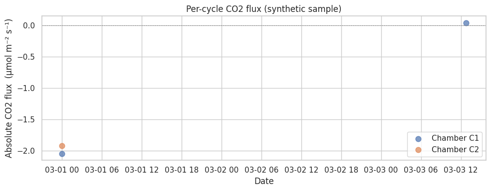
4. Plot the per-cycle flux series

The synthetic sample only produces a handful of cycles (it’s 1 week of toy data). Real LIBZ data yields thousands — try setting PALMWTC_DATA_DIR to a real chamber dataset.

fig, ax = plt.subplots(figsize=(10, 4))
for chamber, group in cycles.groupby("chamber"):
    ax.scatter(
        pd.to_datetime(group["flux_date"]),
        group["flux_absolute"],
        label=f"Chamber {chamber}",
        s=60,
        alpha=0.7,
    )
ax.axhline(0, color="grey", linewidth=0.6, linestyle="--")
ax.set_xlabel("Date")
ax.set_ylabel("Absolute CO2 flux  (μmol m⁻² s⁻¹)")
ax.set_title("Per-cycle CO2 flux (synthetic sample)")
ax.legend()
plt.tight_layout()
plt.show()

5. Cycle-quality summary

qc_flag is the per-cycle pass/fail flag (0 = pass, 1 = warn, 2 = fail). r2 is the linear-fit goodness on the closed-phase concentration ramp; high R² + low NRMSE + appropriate SNR → cycle accepted into calibration windows.

cycles[["chamber", "qc_flag", "r2", "nrmse", "snr"]].groupby("chamber").describe()

	qc_flag								r2		...	nrmse		snr
	count	mean	std	min	25%	50%	75%	max	count	mean	...	75%	max	count	mean	std	min	25%	50%	75%	max
chamber
C1	2.0	0.5	0.707107	0.0	0.25	0.5	0.75	1.0	2.0	0.339095	...	0.210656	0.221757	2.0	2.266499	1.237885	1.391182	1.828841	2.266499	2.704158	3.141816
C2	1.0	1.0	NaN	1.0	1.00	1.0	1.00	1.0	1.0	0.552352	...	0.201954	0.201954	1.0	3.539510	NaN	3.539510	3.539510	3.539510	3.539510	3.539510

2 rows × 32 columns

Next

• 031 / 032 — promote high-confidence cycles into calibration windows (run_step("windows", paths)).

• 033 — validate against literature ecophysiology bounds (run_step("validation", paths)).

• CLI shortcut — palmwtc run runs all four steps end-to-end.